Tutorial on fMRI Test-Retest Reliability Estimation
Published:
This tutorial is based on my presentation at the FMRI Lab meeting on November 26, 2024. You can find the pdf of the talk here.
In fMRI, we calculate statistic measures, e.g., t-, F-statstic, correlation coefficient, for each voxel to generate activation maps. Raw statistic maps are thresholded to give voxels labels with either “active” or “inactive”. In an ideal world, the classification of voxels into active/inactive would be invariant across different trials of the same task. In that case, the classification we yield from thresholding the statistic measure is the ground truth of activation. However, there is always variation of activation maps across different trials of experiment. This is due to, e.g., movement, physiological noise, ambient noise, and most importantly, the neural activity of the subject is not temporal shift invariant. Therefore, it is important to quantify the (test-retest) reliability of the activation maps we get from the acquired fMRI signals.
ROC Curves
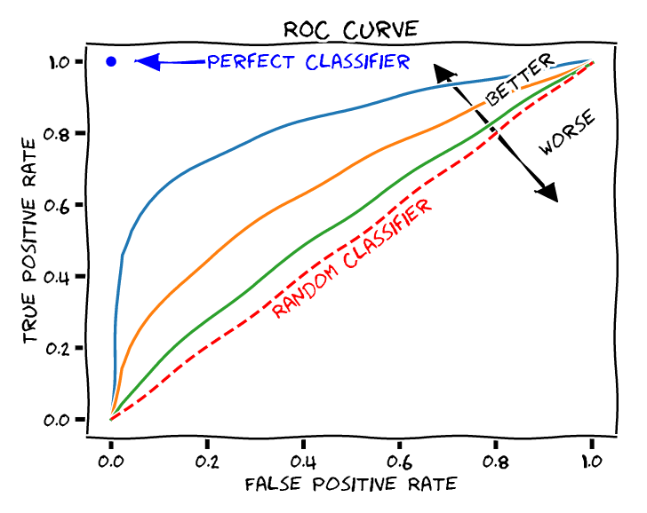
One of the methods for this purpose is to calculate the receiver operating characteristic (ROC) curve.
To get an ROC curve for a, say, t-score map, we sweep the threshold value. For each threshold, calculate (FPR,TPR), get a dot in the ROC curve. 
The definition of false positive rate (FPR) and true positive rate (TPR) are as follow:
Intuitively, you can view FPR and TPR as “false alarm” and “hit”, respectively.
Q:Which one is better: guess all positive, or guess all negative? (suppose in fMRI, proportion of truly activated voxels is far less than 1/2)
A: They are the same! Guessing all positive will be the top-right corner in the ROC plot whereas guessing all negative will be at the bottom-left corner. They corresponding to random classifiers with positive probability $\rho=1$ and $\rho=0$, respectively.
A natural question is: how to know the ground truth activation classification? If we don’t have the ground truth, we can not calculate FP, FN, TP, TN. One straightforward solution may be taking a long scan, with many cycles of the same task, then take the resultant high reliability activation as ground truth. This method is simple but comes with high cost. An alternative way is to use statistic model to estimate the ground truth. Here we introduce a model proposed by Genovese, et al., which I call the mixed-binomial model.
Mixed-binomial Model
Vanilla Case
The mixed-binomial model entails $M\geq 4$ repetitions of the same fMRI experiment. It contains the following major assumptions:
- The behavior of voxels across different trials is independent and identical distribution (i.i.d.);
- The behavior of each voxel is independent of other voxels;
- All voxels behave according to the same probability distribution.
These assumptions are obviously not true in real life. For example, given the clustering nature of activation voxels, the neighbors of a active voxel will have higher probability to be active, thus the second assumption is not true. However, the misfit these assumptions introduce should be negligible in most applications. Weaker assumptions could be made to better fit the reality, interested reader can refer to the original paper.
Now, let’s introduce a few quantities that are essential for this model. The first one is called the raw reliability map $R_v$. It is defined as:
Assume $R_v$ is drawn from a mixture of two binomial distributions:
where $\lambda$ is the proportion of truly active voxels, $p_A$ and $p_I$ are the TPR and FPR, respectively. Due to independence assumption, the likelihood function of parameters $p_A, p_I, \lambda$, only depends on the counts:
All the information of the raw reliability map and thus the inference can be reduced to a simpler quantity, called the histogram vector: $\mathbf{n}=(n_0,n_1,…,n_M)$. The log of the posterier likelihood function of the parameters to be estimated $p_A, p_I, \lambda$ is:
You may recognize that the term inside the logarithm resembles the pmf of a binomial distribution, except that we have dropped the combinatorial factors since they are irrelevant to the parameters. We then estimate the parameters by the method of Maximum Likelihood (ML). This can be easily done by matlab’s optimization toolbox.
Dependent Likelihood Model
The above model is powerful for estimating the reliability of a single classifier. However, in fMRI analysis, we use the same statistic maps (e.g., t-score) to generate a series of reliability maps by selecting 𝐾 different thresholds $\tau_0 <\tau_1<…<\tau_{K-1}$.
These reliability maps are not independent. They should share a common $\lambda$, while at each $\tau_k$, the points $(p_I^{(k)},p_A^{(k)})$ are different, $k=0,…,K-1$. So instead of estimating $3K$ different parameters, we estimate $2K+1$ parameters in total.
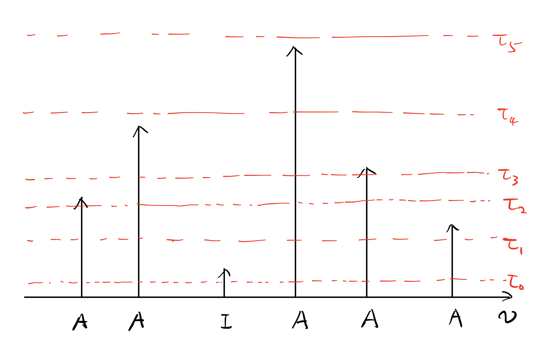
Definition: $p_{Ak}(p_{Ik})$ is the probability that a truly active (inactive) voxel is classified active at $k$ of the threshold levels (it must be the first k thresholds given that the thresholds are arranged in increased order), for $k=0,…,K$. Now I know this quantity could be a bit involved. To help you understand the concept, I prepared an exercise.

Suppose we have 6 voxels in a 1D space, their true labels are marked as “A/I” in Figure 2. The height of each arrow corresponds to the magnitude of the associated statistic measure, e.g., t-score, of each voxel. $K=6$ threshold levels are indicated by the red dashed lines. For the configuration shown in Figure 2, the values of $p_{Ak}$ and $p_{Ik}$ are listed in Table 1.
| k | 0 | 1 | 2 | 3 | 4 | 5 | 6 |
|---|---|---|---|---|---|---|---|
| $p_{Ak}$ | 0 | 0 | 1/5 | 1/5 | 2/5 | 1/5 | 0 |
| $p_{Ik}$ | 0 | 1 | 0 | 0 | 0 | 0 | 0 |
Note that $\sum_{k=0}^{K}p_{Ak}=1, \sum_{k=0}^{K}p_{Ik}=1$. Now define $n_{\mathbf{t}}$ for $\mathbf{t}\triangleq(t_0,…,t_K)$, to be number of voxels classified active at k threshold levels $t_k$ times (out of M) for each $k=0,…,K$. Then the dependent likelihood function is:
The product terms and the outer summation is due to the independent assumptions we made at the beginning. The outer summation sums all the voxels according to the partition given by $n_{\mathbf{t}}$ (voxels with same $n_{\mathbf{t}}$ are grouped together), though in implementation, we simply need to traverse the summation over every voxels. Again, by using ML estimation we can solve the optimal $\mathbf{p_A}=(p_{A0},…,p_{AK}),\mathbf{p_I}=(p_{I0},…,p_{IK})$ and $\lambda$. The actual parameters of interest, $p_A^{(k)}$, i.e., the probability of a truly active voxel being classified active at the $k\text{-th}$ threshold level is $p_A^{(k)}=\sum_{j=k}^{K}p_{Aj}$. This is because, any voxel that is classified k or more than k times out $K$ thresholds must be classified active in the $k\text{-th}$ threshold (since the thresholds are in increasing order), therefore should be included in $p_A^{(k)}$. Similar for $p_{I}^{(k)}=\sum_{j=k}^{K}p_{Ij}$.
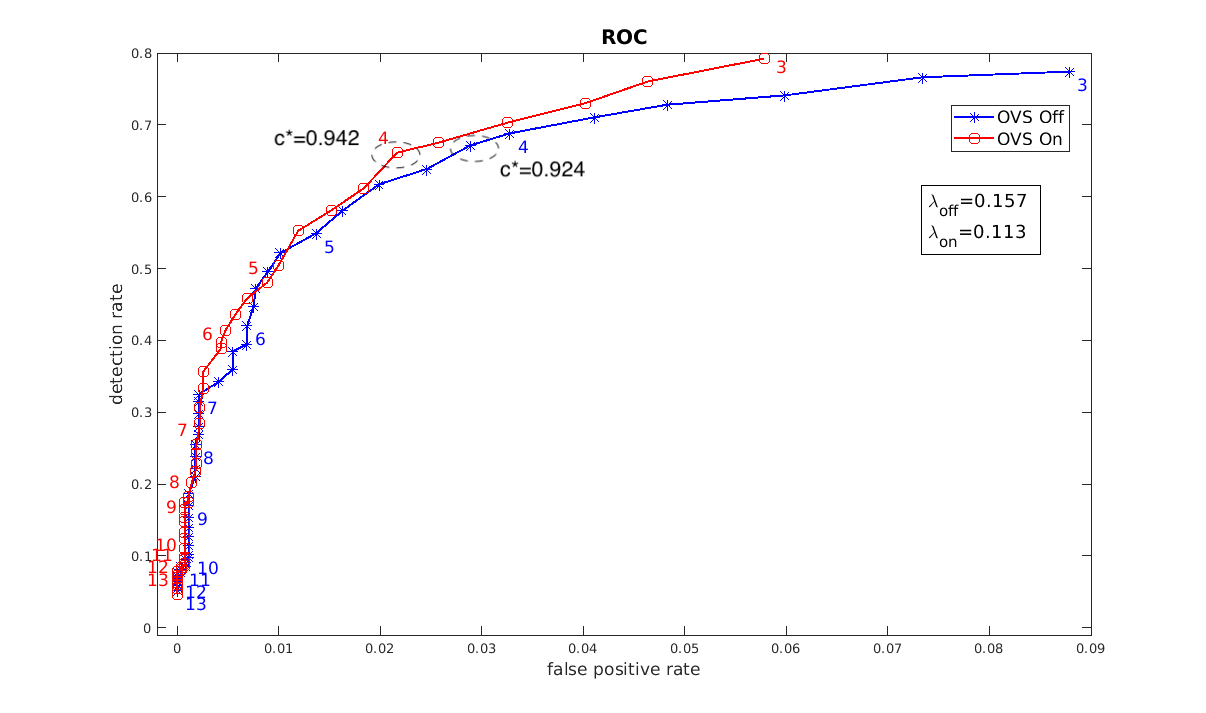
Here is an examplary ROC plot generated accrording to the algorithm described above. 
The numbers indicate the thresholds. The thresholds in the dashed circles are the optimal thresholds that maximize a (subjectively chosen) criterion function $c(\tau)=\lambda p_A(\tau)+(1-\lambda)(1-p_I(\tau))$.
